DistributedSparseGrids.jl

A Julia library implementing an Adaptive Sparse Grid collocation method for integrating memory-heavy objects generated on distributed workers.

For an alternative implementation, see AdaptiveSparseGrids.jl.

Introduction

Efficient methods for the numerical integration (or interpolation) of one-dimensional functions can be directly applied to the multidimensional case via tensor-product constructions. However, the higher the number of dimensions, the less efficient this approach is. A problem which is also known as the curse of dimensionality.

Any integral

$$ \int_{a_1}^{b_1}\cdot\cdot\cdot\int_{a_n}^{b_n} f(x_1,...,x_n) \mathrm{d}x_1\cdot\cdot\cdot\mathrm{d}x_n $$

can be mapped onto the hypercube $[-1,1]^n$ by means of coordinate transformation. Therefore, the problem of integrating multidimensional functions can be studied on the hypercube without loss of generality.

To mitigate the curse of dimensionality that occurs in the integration or interpolation of multidimensional functions on the hypercube, sparse grids use Smolyak's quadrature rule. This is particularly useful if the evaluation of the underlying function is costly. In this library, an Adaptive Sparse Grid Collocation method with a local hierarchical Lagrangian basis, first proposed by Ma and Zabaras (2010), is implemented. For more information about the construction of Sparse Grids, see e.g. Gates and Bittens (2015).

Citing this package

There exists a JOSS paper about this package. You can cite it if you are using this software for academic purposes.

Install

import Pkg
Pkg.add("DistributedSparseGrids")

Implemented features

Nested one-dimensional Clenshaw-Curtis rule
Smolyak's sparse grid construction
local hierarchical Lagrangian basis
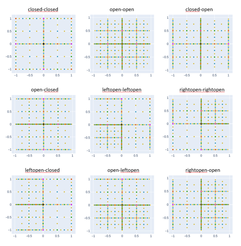
different pointsets (open, closed, halfopen)
adaptive refinement
distributed function evaluation with Distributed.remotecall_fetch
multi-threaded calculation of basis coefficients with Threads.@threads
usage of arbitrary input, collocation point, and return types
integration
experimental: integration over $X_{\sim (i)}$ (the $X_{\sim (i)}$ notation indicates the set of all variables except $X_{i}$).

Usage

General remarks

The quality of the error prediction depends on the number of collocation points. Therefore, for only a few collocation points, adaptive refinement may fail. Therefore it is recommended to generate some initial levels before using adaptive refinement (see examples).
The interpolation is based on a local Lagrangian basis. Functions with discontinuities cannot be approximated.
Sparse grid interpolation and integration will work best with a number of dimension between 1 and 6.
The domain of the sparse grid is always $[-1,1]^n$. The user is responsible to map the input onto this domain.

Point sets

When using sparse grids, one can choose whether the $2d$ second-level collocation points should lay on the boundary of the domain or in the middle between the origin and the boundary. (There are other choices as well.) This results in two different sparse grids, the former with almost all points on the boundary and on the coordinate axes, the latter with all points in the interior of the domain. Since one can choose for both one-dimensional children of the root point individually, there exist a multitude of different point sets for Sparse Grids.

using DistributedSparseGrids
using StaticArrays 

function sparse_grid(N::Int,pointprops,nlevel=6,RT=Float64,CT=Float64)
	# define collocation point
	CPType = CollocationPoint{N,CT}
	# define hierarchical collocation point
	HCPType = HierarchicalCollocationPoint{N,CPType,RT}
	# init grid
	asg = init(AHSG{N,HCPType},pointprops)
	#set of all collocation points
	cpts = Set{HierarchicalCollocationPoint{N,CPType,RT}}(collect(asg))
	# fully refine grid nlevel-1 times
	for i = 1:nlevel-1
		union!(cpts,generate_next_level!(asg))
	end
	return asg
end

# define point properties 
#	1->closed point set
# 	2->open point set
#	3->left-open point set
#	4->right-open point set

asg01 = sparse_grid(1, @SVector [1]) 
asg02 = sparse_grid(1, @SVector [2]) 
asg03 = sparse_grid(1, @SVector [3]) 

asg04 = sparse_grid(2, @SVector [1,1]) 
asg05 = sparse_grid(2, @SVector [2,2]) 
asg06 = sparse_grid(2, @SVector [1,2]) 
asg07 = sparse_grid(2, @SVector [2,1]) 
asg08 = sparse_grid(2, @SVector [3,3]) 
asg09 = sparse_grid(2, @SVector [4,4]) 
asg10 = sparse_grid(2, @SVector [3,1]) 
asg11 = sparse_grid(2, @SVector [2,3]) 
asg12 = sparse_grid(2, @SVector [4,2])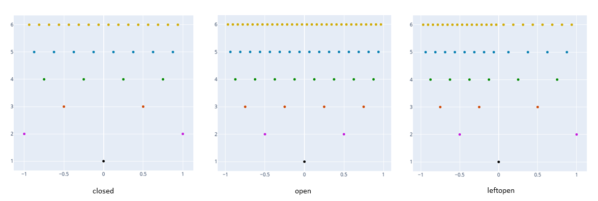

Integration and Interpolation

asg = sparse_grid(4, @SVector [1,1,1,1]) 

#define function: input are the coordinates x::SVector{N,CT} and an unique id ID::String (e.g. "1_1_1_1")
fun1(x::SVector{N,CT},ID::String) = sum(x.^2)

# initialize weights
@time init_weights!(asg, fun1)

# integration
integrate(asg)

# interpolation
x = rand(4)*2.0 .- 1.0
val = interpolate(asg,x)

Distributed function evaluation

asg = sparse_grid(4, @SVector [1,1,1,1]) 

# add worker and register function to all workers
using Distributed
addprocs(2)
ar_worker = workers()
@everywhere begin
    using StaticArrays
    fun2(x::SVector{4,Float64},ID::String) = 1.0
end

# Evaluate the function on 2 workers
distributed_init_weights!(asg, fun2, ar_worker)

Using custom return types

For custom return type T to work, following functions have to be implemented

import Base: +,-,*,/,^,zero,zeros,one,ones,copy,deepcopy

+(a::T, b::T) 
+(a::T, b::Float64) 
*(a::T, b::Float64) 
-(a::T, b::Matrix{Float64})
-(a::T, b::Float64) 
zero(a::T) 
zeros(a::T) 
one(a::T) 
one(a::T) 
copy(a::T)
deepcopy(a::T)

This is already the case for many data types. Below RT=Matrix{Float64} is used.

# sparse grid with 5 dimensions and levels
pointprops = @SVector [1,2,3,4,1]
asg = sparse_grid(5, pointprops, 6, Matrix{Float64}) 

# define function: input are the coordinates x::SVector{N,CT} and an unique id ID::String (e.g. "1_1_1_1_1_1_1_1_1_1"
# for the root poin in five dimensions)
fun3(x::SVector{N,CT},ID::String) = ones(100,100).*x[1]

# initialize weights
@time init_weights!(asg, fun3)

In-place operations

There are many mathematical operations executed which allocate memory while evaluting the hierarchical interpolator. Many of these allocations can be avoided by additionally implementing the inplace operations interface for data type T.

import LinearAlgebra, AltInplaceOpsInterface 

LinearAlgebra.mul!(a::T, b::Float64) 
LinearAlgebra.mul!(a:T, b::T, c::Float64)
AltInplaceOpsInterface.add!(a::T, b::T) 
AltInplaceOpsInterface.add!(a::T, b::Float64) 
AltInplaceOpsInterface.minus!(a::T, b::Float64) 
AltInplaceOpsInterface.minus!(a::T, b::T) 
AltInplaceOpsInterface.pow!(a::T, b::Float64)

For Matrix{Float64} this interface is already implemented.

# initialize weights
@time init_weights_inplace_ops!(asg, fun3)

Distributed function evaluation and in-place operations

# initialize weights
@time distributed_init_weights_inplace_ops!(asg, fun3, ar_worker)

Adaptive Refinement

# Sparse Grid with 4 initial levels
pp = @SVector [1,1]
asg = sparse_grid(2, pp, 4)

# Function with curved singularity
fun1(x::SVector{2,Float64},ID::String) =  (1.0-exp(-1.0*(abs(2.0 - (x[1]-1.0)^2.0 - (x[2]-1.0)^2.0) +0.01)))/(abs(2-(x[1]-1.0)^2.0-(x[2]-1.0)^2.0)+0.01)

init_weights!(asg, fun1)

# adaptive refine
for i = 1:20
# call generate_next_level! with tol=1e-5 and maxlevels=20
cpts = generate_next_level!(asg, 1e-5, 20)
init_weights!(asg, collect(cpts), fun1)
end

# plot
import PlotlyJS
surfplot = PlotlyJS.surface(asg, 100)
gridplot = PlotlyJS.scatter3d(asg)
PlotlyJS.plot([surfplot, gridplot])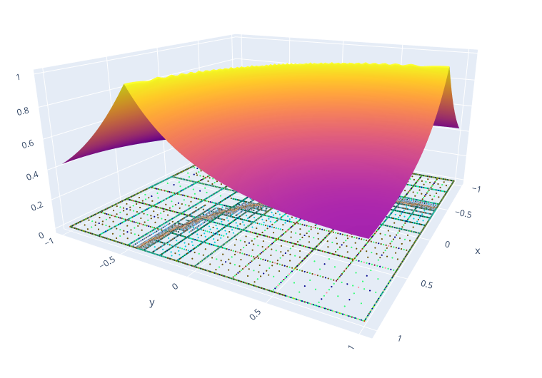

Plotting

1d

# grid plots
PlotlyJS.scatter(sg::AbstractHierarchicalSparseGrid{1,HCP}, lvl_offset::Bool=false; kwargs...) 
UnicodePlots.scatterplot(sg::AbstractHierarchicalSparseGrid{1,HCP}, lvl_offset::Bool=false)

# response function plots
UnicodePlots.lineplot(asg::AbstractHierarchicalSparseGrid{1,HCP}, npts = 1000, stoplevel::Int=numlevels(asg))
PlotlyJS.surface(asg::SG, npts = 1000, stoplevel::Int=numlevels(asg); kwargs...)

2d

# grid plots
PlotlyJS.scatter(sg::AbstractHierarchicalSparseGrid{2,HCP}, lvl_offset::Float64=0.0, color_order::Bool=false) 
UnicodePlots.scatterplot(sg::AbstractHierarchicalSparseGrid{2,HCP})
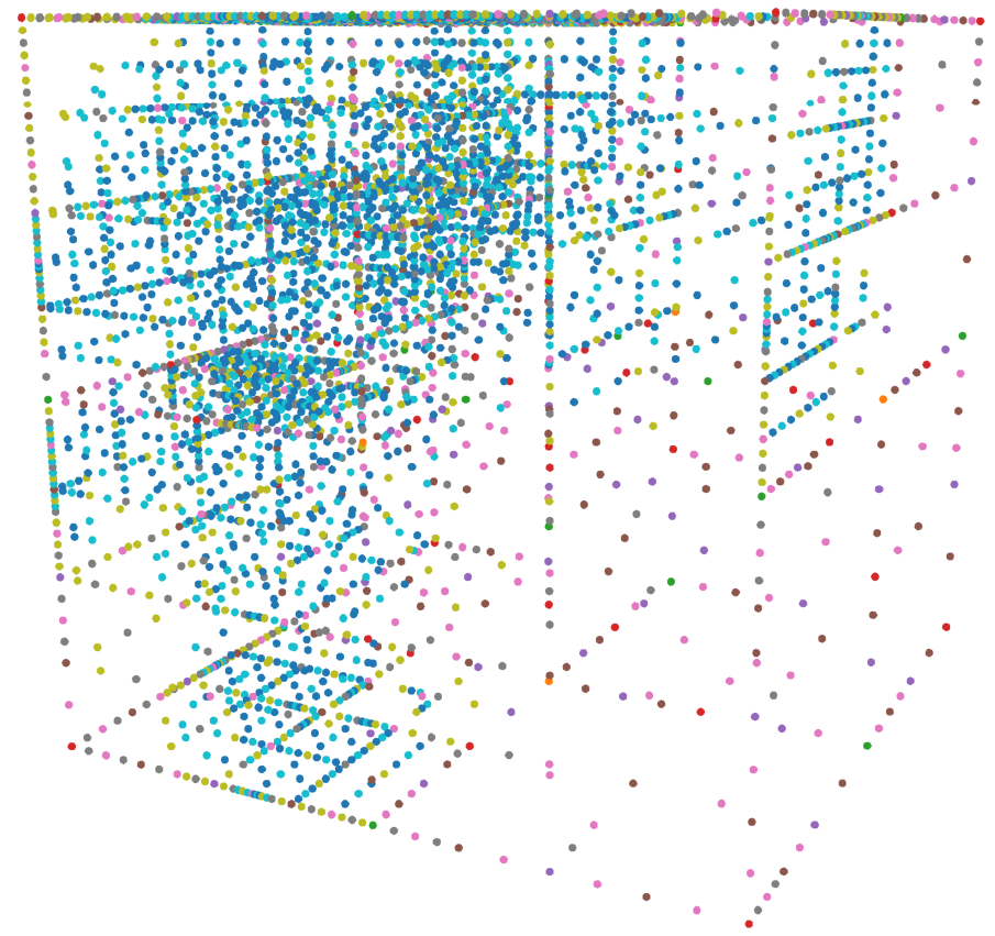
PlotlyJS.scatter3d(sg::AbstractHierarchicalSparseGrid{2,HCP}, color_order::Bool=false, maxp::Int=1)

# response function plot
PlotlyJS.surface(asg::AbstractHierarchicalSparseGrid{2,HCP}, npts = 20; kwargs...)

3d

# grid plot
PlotlyJS.scatter3d(sg::AbstractHierarchicalSparseGrid{3,HCP}, color_order::Bool=false, maxp::Int=1)

Next steps

nonlinear basis functions
wavelet basis

Contributions, report bugs and support

Contributions to or questions about this project are welcome. Feel free to create a issue or a pull request on GitHub.