This repo contain the code to make Fisher contour plots.

Using FisherPlot.jl is quite easy.

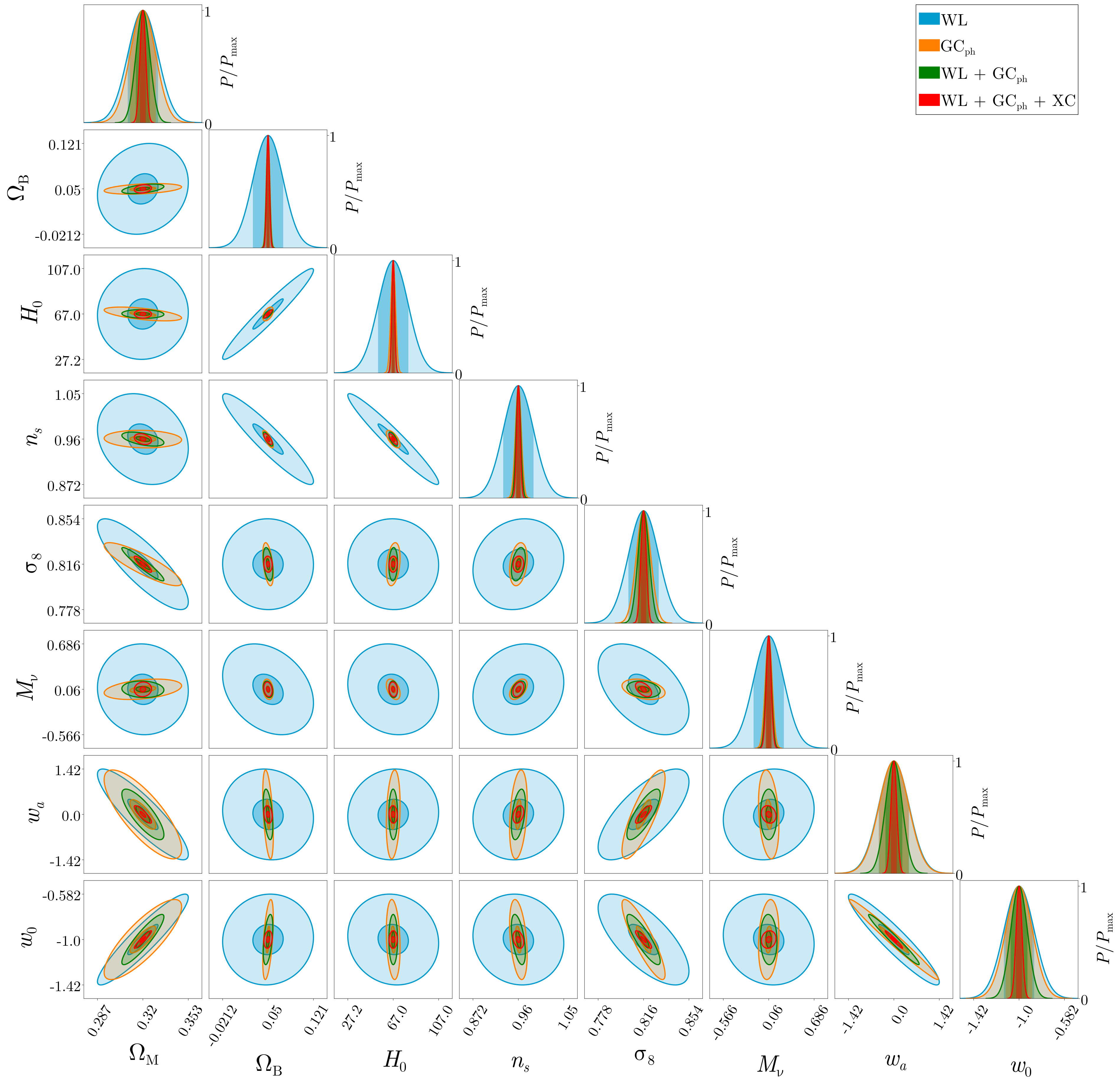
Let us start defining some arrays containing:

• the string identifying the parameters we want to plot
• the central values for the parameters involved in the analysis
• the probes analyzes (necessary for the legend)
• the color for each probe

LaTeXArray = [L"\Omega_\mathrm{M}", L"\Omega_\mathrm{B}", L"H_0", ...]
central_values =[0.32, 0.05, 67., ...]
probes = [L"\mathrm{WL}", L"\mathrm{GC}_\mathrm{ph}", ...]
colors = ["deepskyblue3", "darkorange1", ...]

The second object to instantiate is a Dict containing the following keys:

PlotPars = Dict("sidesquare" => 400,
"dimticklabel" => 50,
"parslabelsize" => 80,
"textsize" => 80,
"PPmaxlabelsize" => 60,
"font" => font,
"xticklabelrotation" => 45.)

where font is necessary to use LaTeX in all plots and should something similar to

FisherPlot.assetpath("/usr/share/fonts/computer_modern", "NewCM10-Regular.otf")

The last two object to instantiate are two 2D arrays:

• limits, which contains the lower (limits[i,1]) and the lower (limits[i,2]) limit for plotting the i-th parameter
• ticks, which contains the lower (ticks[i,1]) and the lower (ticks[i,2]) point where put a tick for the i-th parameter

We have almost done, we just need to use two commands, the first being:

canvas = FisherPlot.preparecanvas(LaTeX_array, limits, ticks, probes, colors, PlotPars::Dict)

which prepare a white canvas where we are going to paint our Fisher matrices contours. The last command (which must be repeated for each Fisher correlation matrix we want to plot) is:

FisherPlot.paintcorrmatrix!(canvas, central_values, correlation_matrix, "deepskyblue3")