SerialDependence.jl

When dealing with categorical data, things like autocorrelation function are not defined. This is what this module is for : computing categorical serial dependences.

Travis	Appveyor

The module mostly implements the methods described in C. Weiss's book "An Introduction to Discrete-Valued Time Series" (2018) [1], with some extras. It contains three main functions :

All the module's functions require a 'lag's input : 'lags' can be an Int, or an Array{Int,1} if you want to do a serial dependence plot. The function then returns a Float64 or an Array{Float64,1} depending on 'lags' being an Int or Array{Int,1}.

• cramer_coefficient(series, lags): measures average association between elements of 'series' at time t and time t + lags. Cramer's k is an unsigned measurement : its values lies in [0,1], 0 being perfect independence and 1 perfect dependence. k can be bias, for more infos, refer to [1].

• cohen_coefficient(series, lags): measures average agreement between elements of 'series' at time t and time t + lags.
  Cohen's k is a signed measurement : its values lie in [-pe/(1 -pe), 1], with positive (negative) values indicating positive (negative) serial dependence at 'lags'. pe is probability of agreement by chance.

• theils_u(series, lags): measures average portion of information known about 'series' at t + lags given that 'series' is known at time t. U is an unsigned measurement: its values lies in [0,1], 0 meaning no information shared and 1 complete knowledge (determinism).

• bootstrap_CI(Series, lags, coef_func, n_iter = 1000): Returns top and bottom limit for a 95% confidence interval at values of 'lags'.
  • 'coef_func' is the function for which the CI needs to be computed. Possible values : 'cramer_coefficient, cohen_coefficient, theils_u'.
  • 'n_iter' controls how many iterations are run during the bootstrap process. Large 'n_iter', means more precision but also more compute time.
• rate_evolution(Series): This is a visual test of "stationarity" : if it varies linearly, then the time-series can be considered as stationary. Returns an array of array. Each of the internal array represents one of the categories in 'Series'and describes it's evolution rate.

Using the pewee birdsong data (1943) one can do a serial dependence plot using Cohen's cofficient as follow :

using DelimitedFiles
using SerialDependence
using Plots
#reading 'pewee' time-series test folder.
series = readdlm("test\\pewee.txt",',')[1,:] 
lags = collect(1:25)
v = cohen_coefficient(series, lags)
t, b = bootstrap_CI(series, cramer_coefficient, lags)
a = plot(lags, v, xlabel = "Lags", ylabel = "K", label = "Cramer's k")
plot!(a, lags, t, color = "red", label = "Limits of 95% CI"); plot!(a, lags, b, color = "red", label = "")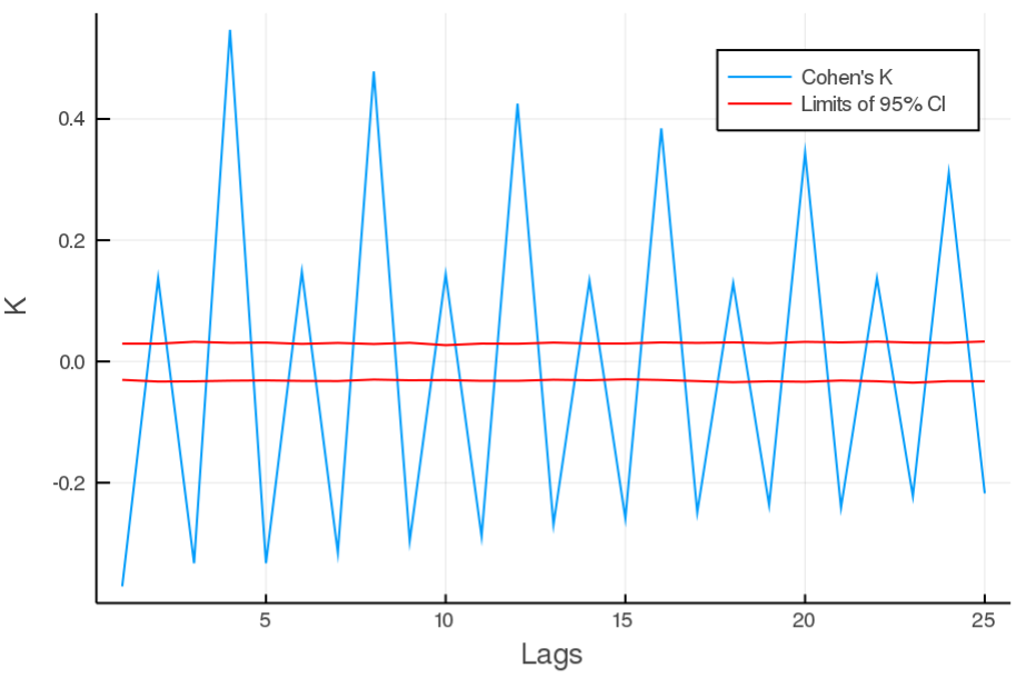

[] Implement bias correction for cramer's v

[1] DOI : 10.1002/9781119097013