FEniCS.jl: Finite Element PDE Solving in Julia

FEniCS.jl is a wrapper for the FEniCS library for finite element discretizations of PDEs. This wrapper includes three parts:

1. Installation and direct access to FEniCS via a Conda installation. Alternatively, one may use their current FEniCS installation.
2. A low-level development API and provides some functionality to make directly dealing with the library a little bit easier, but still requires knowledge of FEniCS itself. Interfaces have been provided for the main functions and their attributes, and instructions to add further ones can be found here.
3. A high-level API for usage with DifferentialEquations. An example can be seen solving the heat equation with high order adaptive timestepping.

Various gists/jupyter notebooks have been created to provide a brief overview of the overall functionality, and of any differences between the Pythonic FEniCS and the Julian wrapper. DifferentialEquations.jl ecosystem. Paraview can also be used to visualize various results, just like in FEniCS (see below).

To get the wrapper on your system, providing a FEniCS installation exists, follow the below steps:

1. Add PyCall with the correct Python environment corresponding to FEniCS. Then simply add FEniCS.jl using Pkg.add("FEniCS")

2. Alternatively, one can install Docker and then run the following command

docker run -ti cmhyett/julia-fenics

and once inside, Julia can be accessed by calling

julia

Once inside the Julia environment, simply add FEniCS with Pkg.add("FEniCS"). All other dependencies are handled by the docker image.

This wrapper was originally started via the Google Summer of Code program along with the help of Chris Rackauckas and Bart Janssens. This was continued via GSoC '18 along with the help of Chris Rackauckas and Timo Betcke.

Below is a small demonstration of how a user would use our code to solve the Poisson equation with Dirichlet conditions. This directly mirrors one of the tutorials FEniCS provides

using FEniCS
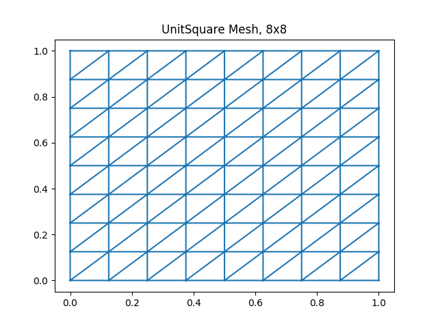
mesh = UnitSquareMesh(8,8)
V = FunctionSpace(mesh,"P",1)
u_D = Expression("1+x[0]*x[0]+2*x[1]*x[1]", degree=2)
u = TrialFunction(V)
bc1 = DirichletBC(V,u_D, "on_boundary")
v = TestFunction(V)
f = Constant(-6.0)
a = dot(grad(u),grad(v))*dx
L = f*v*dx
U = FeFunction(V)
lvsolve(a,L,U,bc1) #linear variational solver
errornorm(u_D, U, norm="L2")
get_array(L) #this returns an array for the stiffness matrix
get_array(U) #this returns an array for the solution values
vtkfile = File("poisson/solution.pvd")
vtkfile << U.pyobject #exports the solution to a vtkfile

We can also plot the solution (this relies on FEniCS backend for plotting) or import it from our file into Paraview:

import PyPlot # plotting won't work if PyPlot is not imported
FEniCS.Plot(U)
FEniCS.Plot(mesh)

See the examples directory for more examples.