MicroCanonicalHMC.jl

A Julia implementation of Micro-Canonical HMC. You can checkout the JAX version here.

Features

GPU support through CUDA.jl
Integrated within Turing.jl ecosystem.

How to use it

Define the Model

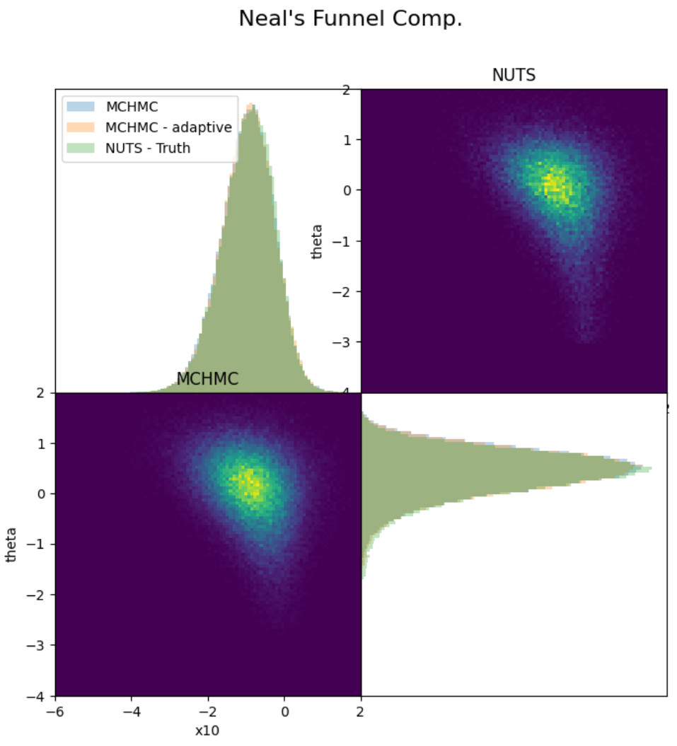
Start by drawing a Neal's funnel model in Turing.jl:

# The statistical inference frame-work we will use
using Turing
using Random
using PyPlot
using LinearAlgebra
using MicroCanonicalHMC

d = 21
@model function funnel()
    θ ~ Normal(0, 3)
    z ~ MvNormal(zeros(d-1), exp(θ)*I)
    x ~ MvNormal(z, I)
end

(; x) = rand(funnel() | (θ=0,))
funel_model = funnel() | (; x);

Define the Sampler

nadapt = 10_000
TEV = 0.001
spl = MCHMC(nadapt, TEV)

The first two entries mean that the step size and the trajectory length will be self-tuned. In the ensemble sampler, the third number represents the number of workers. VaE_wanted sets the hamiltonian error per dimension that will be targeted. Fixing sigma=ones(d) avoids tunin the preconditioner.

Start Sampling

samples_mchmc = sample(funel_model, externalsampler(spl), 100_000)

Compare to NUTS

samples_hmc = sample(funnel_model, NUTS(5_000, 0.95), 50_000)

NUTS effective samples per second --> ~630
MCHMC effective samples per second --> ~1340
Ensemble MCHMC effective samples per second per worker --> ~957

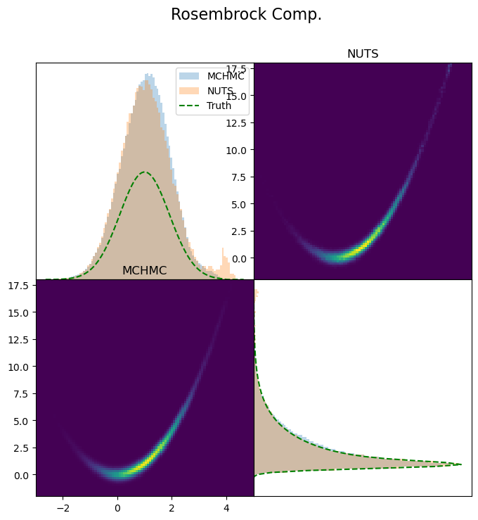
Using your own likelihood function

Define a Target

Start by defining your likelihood function and its gradient

d=2
function ℓπ(x; a=a, b=b)
    x1 = x[1:Int(d / 2)]
    x2 = x[Int(d / 2)+1:end]
    m = @.((a - x1)^2 + b * (x2 - x1^2)^2)
    return -0.5 * sum(m)
end
function ∂lπ∂θ(x)
    return ℓπ(x), ForwardDiff.gradient(ℓπ, x)
end
θ_start = rand(MvNormal(zeros(d), ones(d)))

Wrap it into a CustomTarget

target = CustomTarget(ℓπ, ∂lπ∂θ, θ_start)

Start Sampling

samples_mchmc = Sample(spl, target, 500_000; dialog=true);