Implicit 3D Plots

Visualizing parametrized space curves or surfaces is not complicated: We simply need to iterate the parametrization's domain (usually ) and get a reasonably smooth plot as a result. Implicitly defined surfaces and curves pose a problem however: If we were to proceed in a similar manner, we would have to iterate through and check, whether the implicit equations are 0 in any of the points. This approach is problematic in two ways. Firstly, numerics and potentially instable implicit functions prohibit this method: It is unlikely, that we will find rational points that actually lie on the curve or surface in this way. Generally, this method will only yield points that approximately lie on the implicit set. However, this we could cope with: the grid can be chosen arbitrarily small, so thoretically we could reach machine presision with this method - at the expense of a reasonable runtime. More problematically however, there is no natural notion of what point comes next on the curve or surface. In the case of parametrized curves, we always know the next point on the curve, because there is a natural total order on . Finding the next point on an implicit curve is harder, as the proximity of points is an insufficient criterion in this setting and the closest point might not be unique.

Drawing inspiration from the Julia package ImplicitPlots.jl there is a way out from this dilemma though. Using the library Meshing.jl immediately enables us to sample an implicit surface and form a mesh between the points that covers the surface. For implicit space curves, let us recall that since a space curve can be represented by two equations, we can simply intersect the two corresponding surfaces to obtain an approximation. For this reason, we can utilize the previously mentioned meshes and intersect them. Afterwards, Makie.jl is utilized to visualize the outcome.

Installation

julia> ]
(@v1.7) pkg> add Implicit3DPlotting

Usage

There are two main methods in this package: plot_implicit_surface and plot_implicit_curve. Let us first consider an example of the former:

julia> f(x) = x[1]^2+x[2]^2-x[3]^2-1
julia> scene = plot_implicit_surface(f; transparency=false, xlims=(-3,3), ylims=(-3,3), zlims=(-3,3))

The result of this can be seen in the following image:

Notice that the standard options are that the plot's color is :steelblue, the plot is transparent, the surface's shading is activated, the standard meshing method is MarchingCubes, because it is slightly faster than MarchingTetrahedra, and the standard search domain is the hypercube [-3,3]^3 per default. All these settings can be changed in the package's methods. All possible options are listed at the end of the README file.

As an example of the plot_implicit_curve, let us consider the input

julia> f(x)=x[1]^2+x[2]^2-x[3]^2-1
julia> g(x)=x[1]^2+x[2]^2+x[3]^2-2
julia> plot_implicit_curve(f, g)

which produces the following picture:

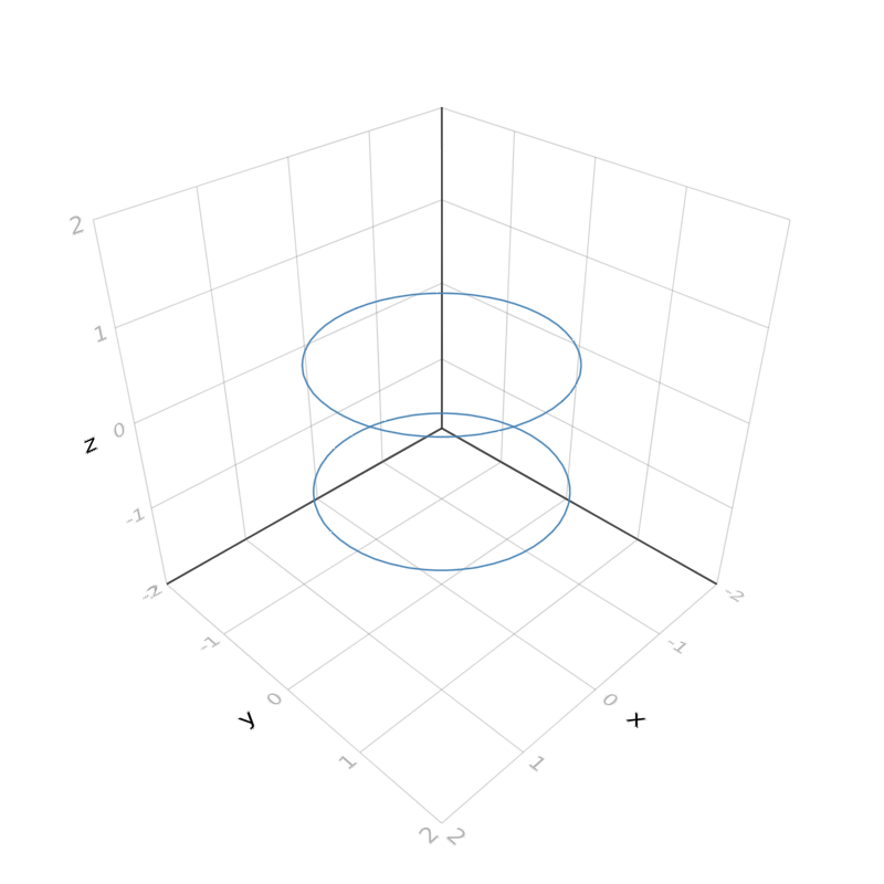
In this context, it is important to notice that the two implicit surfaces generated by the implicit equations need to lie in relative general position. If they are only kissing, the mesh might not be able to reflect their intersection properly.

Since the 0.1.7 update, it is possible to use different Makie backends. In particular, the OpenGL-based backend GLMakie and the WebGL-based backend WGLMakie are admissible. The default is GLMakie. They can be called via the boolean input WGLMode that is accepted by all exported methods by the package Implicit3DPlotting:

julia> plot_implicit_surface(f; WGLMode=false) # to use the GLMakie backend
julia> plot_implicit_curve(f, g; WGLMode=true) # to use the WGLMakie backend

Options

The options that can be changed in the methods for plotting 3D curves and surfaces are given below. They should be added after the semicolon in the methods plot_implicit_curve or plot_implicit_surface, e.g. as follows: plot_implicit_surface(f; kwargs...).

• xlims, ylims and zlims are vectors that determine the search domain for the meshing algorithms: xlims = (-3,3),
• color = :steelblue,
• For surfaces: transparency = true,
• For surfaces: shading = true,
• For surfaces: Do we want the plot to be displayed as a 1-skeleton (wireframe) or a surface? wireframe = false,
• For surfaces: Add a color map dependent on the surface's -value by zcolormap = :viridis (for other color schemes, see https://docs.juliaplots.org/latest/generated/colorschemes/),
• Marching tetrahedra or marching cubes? MarchingModeIsCubes = true,
• Samples determine the accuracy of the plot's display. The higher the sampling numbers, the better. samples=(35,35,35),
• Display axes? show_axis = true,
• resolution=(800,800),
• scale_plot=false,
• Should the plot be displayed in-line or in an external window? in_line=false,
• For curves: How thick should the linestroke be? linewidth = 1.5,
• We can rescale the plot with scaling = (x,y,z),
• Other GLMakie-based kwargs... (see https://makie.juliaplots.org/stable/).