![]()
This package provides tools to create and plot vortex filaments and to compute the velocity they induce in three dimensions with support for infinite and semi-infinite vortex filaments.
VortexFilaments.jl is registered in the general Julia registry. To install, type e.g.,
] add VortexFilamentsThen, in any version, type
using VortexFilamentsThe package introduces the VortexFilament type, which represents a vortex filament that is discretized with vertices and segments connecting those vertices. A vortex filament can be created by calling the provided constructor,
vertices = [[0.0,0.0,0.0], [0.0,1.0,0.0], [1.0,1.0,0.0], [1.0,0.0,0.0]]
Γ = 1.0 # strength of the vortex filament
vf = VortexFilament(Γ,vertices)
which can then be plotted with the provided type recipe.
plot(vf)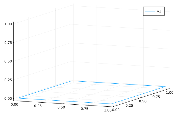
The velocity that the vortex filament vf induces at a location x can be computed using as inducevelocity(vf,x), which returns a 3-element vector representing the velocity vector.
x = [0.5,0.5,0.5]
inducevelocity(vf,x)
If you don't want the filament to be closed, provide the constructor with the keyword isclosed=false.
vf = VortexFilament(Γ,vertices,isclosed=false)
plot(vf)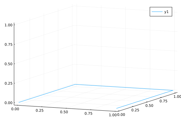
The vortex filament can also be an infinite vortex filament or a semi-infinite vortex element. If you want to plot these filaments, you have to provide the plot axis limits for the direction in which the vortex filament extends to infinity.
vertices = [[-Inf,0.0,0.0], [Inf,0.0,0.0]]
Γ = 1.0 # strength of the vortex filament
vf = VortexFilament(Γ,vertices) # infinite vortex filament
plot(vf,xlims=[-2,2],ylims=[-2,2])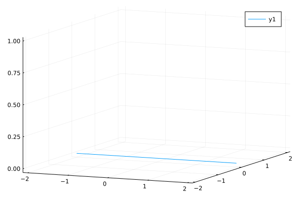
vertices = [[0,0.0,0.0], [Inf,0.0,0.0]]
Γ = 1.0 # strength of the vortex filament
vf = VortexFilament(Γ,vertices) # semi-infinite vortex filament
plot(vf,xlims=[-2,2],ylims=[-2,2])
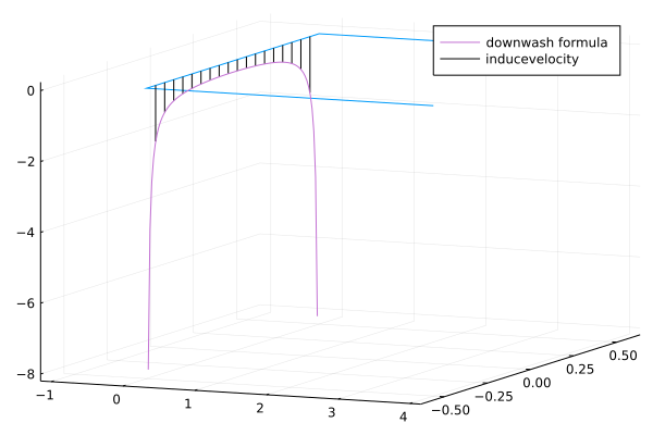
These (semi-)infinite filaments also work with the inducevelocity method. This provides the possibility to model a horseshoe vortex.
b = 1
Γ = 1.0 # sign depends on the order of the vertices
v1 = [Inf,-b/2,0]
v2 = [0,-b/2,0]
v3 = [0,b/2,0]
v4 = [Inf,b/2,0]
vf = VortexFilament(Γ,[v1,v2,v3,v4])
yrange1 = range(-b/2,b/2,length=20)
xevals = [[0.0,y,0.0] for y in yrange1[2:end-1]];
w = inducevelocity.(Ref(vf),xevals);
We will compare the induced velocity with the formula for the downwash for a horseshoe vortex.
yrange2 = range(-b/2,b/2,length=100)
downwash(Γ,b,y) = -Γ/(4π)*b/((b/2)^2-y^2);
wvec = [[xevals[i],xevals[i]+w[i]] for i in 1:length(w)];
p = plot(vf,xlims=[-1,4],ylims=[-0.6*b,0.6*b],label=false)
for i in 1:length(wvec)
plot3d!((v->v[1]).(wvec[i]),(v->v[2]).(wvec[i]),(v->v[3]).(wvec[i]),color=:black,label=false)
end
plot3d!(zeros(length(yrange2)),yrange2,downwash.(1.0,b,yrange2),label="downwash formula")
plot!([],[],c=:black,label="inducevelocity")