MultiScaleArrays.jl

A framework for developing multi-scale arrays for use in scientific machine learning (SciML) simulations
Author SciML
Popularity
45 Stars
Updated Last
2 Years Ago
Started In
October 2016

MultiScaleArrays

Join the chat at https://gitter.im/JuliaDiffEq/Lobby Build Status Coverage Status codecov

MultiScaleArrays.jl allows you to easily build multiple scale models which are fully compatible with native Julia scientific computing packages like DifferentialEquations.jl or Optim.jl. These models utilize a tree structure to describe phenomena of multiple scales, but the interface allows you to describe equations on different levels, using aggregations from lower levels to describe complex systems. Their structure allows for complex and dynamic models to be developed with only a small performance difference. In the end, they present themselves as an AbstractArray to standard solvers, allowing them to be used in place of a Vector in any appropriately made Julia package.

Example

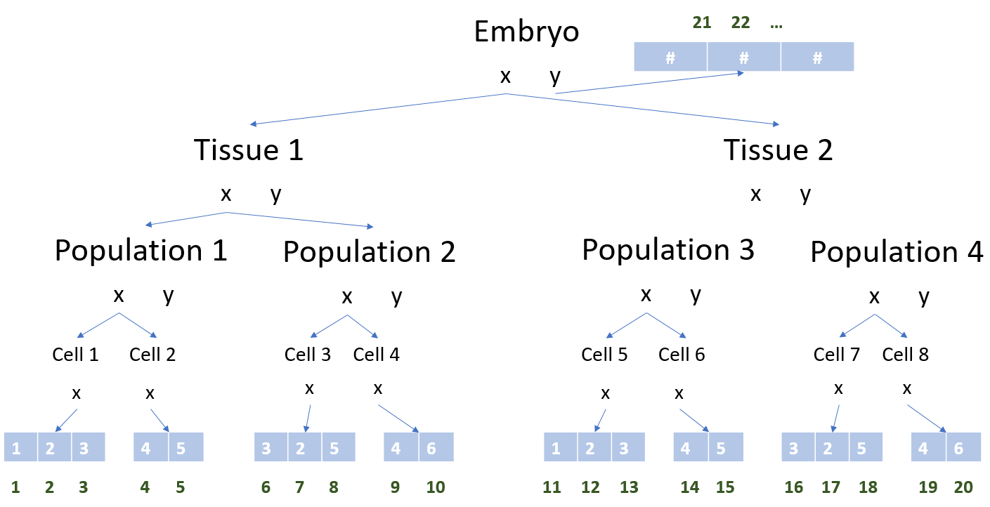
The usage is best described by an example. Here we build a hierarchy where Embryos contain Tissues which contain Populations which contain Cells, and the cells contain proteins whose concentrations are modeled as simply a vector of numbers (it can be anything linearly indexable).

using MultiScaleArrays
struct Cell{B} <: AbstractMultiScaleArrayLeaf{B}
    values::Vector{B}
end
struct Population{T<:AbstractMultiScaleArray,B<:Number} <: AbstractMultiScaleArray{B}
    nodes::Vector{T}
    values::Vector{B}
    end_idxs::Vector{Int}
end
struct Tissue{T<:AbstractMultiScaleArray,B<:Number} <: AbstractMultiScaleArray{B}
    nodes::Vector{T}
    values::Vector{B}
    end_idxs::Vector{Int}
end
struct Embryo{T<:AbstractMultiScaleArray,B<:Number} <: AbstractMultiScaleArrayHead{B}
    nodes::Vector{T}
    values::Vector{B}
    end_idxs::Vector{Int}
end

This setup defines a type structure which is both a tree and an array. A picture of a possible version is the following:

Let's build a version of this. Using the constructors we can directly construct leaf types:

cell1 = Cell([1.0; 2.0; 3.0])
cell2 = Cell([4.0; 5.0])

and build types higher up in the hierarchy by using the constuct method. The method is construct(T::AbstractMultiScaleArray, nodes, values), though if values is not given it's taken to be empty.

cell3 = Cell([3.0; 2.0; 5.0])
cell4 = Cell([4.0; 6.0])
population  = construct(Population, deepcopy([cell1, cell3, cell4]))
population2 = construct(Population, deepcopy([cell1, cell3, cell4]))
population3 = construct(Population, deepcopy([cell1, cell3, cell4]))
tissue1 = construct(Tissue, deepcopy([population, population2, population3])) # Make a Tissue from Populations
tissue2 = construct(Tissue, deepcopy([population2, population, population3]))
embryo = construct(Embryo, deepcopy([tissue1, tissue2])) # Make an embryo from Tissues

Human readable printing of the embryo structure

print_human_readable(embryo)
# +|Tissue;                                                 |Tissue                                                 
#  +|Popula;           |Popula;           |Popula;          +|Popula;           |Popula;           |Popula          
#   +Cell; Cell; Cell; +Cell; Cell; Cell; +Cell; Cell; Cell; +Cell; Cell; Cell; +Cell; Cell; Cell; +Cell; Cell; Cell

print_human_readable(embryo;NcharPerName=2)
# +|Ti;                                   |Ti                                   
#  +|Po;         |Po;         |Po;        +|Po;         |Po;         |Po        
#   +Ce; Ce; Ce; +Ce; Ce; Ce; +Ce; Ce; Ce; +Ce; Ce; Ce; +Ce; Ce; Ce; +Ce; Ce; Ce

Here, if the 'AbstractMultiScaleArrayLeaf's contain several fields, you can specify them with fields = [field1,field2,...]

print_human_readable(embryo;NcharPerName=2,fields=[:values])
# +|Ti;                                                                                                                                                                             |Ti                                                                                                                                                                             
#  +|Po;                                                       |Po;                                                       |Po;                                                      +|Po;                                                       |Po;                                                       |Po                                                      
#   +va: [1.0, 2.0, 3.0]; va: [3.0, 2.0, 5.0]; va: [4.0, 6.0]; +va: [1.0, 2.0, 3.0]; va: [3.0, 2.0, 5.0]; va: [4.0, 6.0]; +va: [1.0, 2.0, 3.0]; va: [3.0, 2.0, 5.0]; va: [4.0, 6.0]; +va: [1.0, 2.0, 3.0]; va: [3.0, 2.0, 5.0]; va: [4.0, 6.0]; +va: [1.0, 2.0, 3.0]; va: [3.0, 2.0, 5.0]; va: [4.0, 6.0]; +va: [1.0, 2.0, 3.0]; va: [3.0, 2.0, 5.0]; va: [4.0, 6.0]

if your screen is small, then print a sub-part of the AbstractMultiScaleArray:

print_human_readable(embryo.nodes[1].nodes[1];fields=[:values])
# +values: [1.0, 2.0, 3.0]; values: [3.0, 2.0, 5.0]; values: [4.0, 6.0]

Indexing and Iteration

The head node then acts as the king. It is designed to have functionality which mimics a vector in order for usage in DifferentialEquations or Optim. So for example

embryo[12]

returns the "12th protein", counting by Embryo > Tissue > Population > Cell in order of the vectors. The linear indexing exists for every AbstractMultiScaleArray. These types act as full linear vectors, so standard operations do the sensical operations:

embryo[10] = 4.0 # changes protein concentration 10
embryo[2,3,1] # Gives the 1st cell in the 3rd population of the second tissue
embryo[:] # generates a vector of all of the protein concentrations
eachindex(embryo) # generates an iterator for the indices

Continuous models can thus be written at the protein level and will work seamlessly with DifferentialEquations or Optim which will treat it like a vector of protein concentrations. Using the iterators, note that we can get each cell population by looping through 2 levels below the top, so

for cell in level_iter(embryo,3)
  # Do something with the cells!
end

or the multiple level iter, which is the one generally used in DifferentialEquations.jl functions:

for (cell, dcell) in LevelIter(3,embryo, dembryo)
    # If these are similar structures, `cell` and `dcell` are the similar parts
    cell_ode(dcell,cell,p,t)
end

LevelIterIdx can give the indices along with iteration:

for (cell, y, z) in LevelIterIdx(embryo, 3)
    # cell = embryo[y:z]
end

However, the interesting behavior comes from event handling. Since embryo will be the "vector" for the differential equation or optimization problem, it will be the value passed to the event handling. MultiScaleArrays includes behavior for changing the structure. For example:

tissue3 = construct(Tissue, deepcopy([population, population2]))
add_node!(embryo, tissue3) # Adds a new tissue to the embryo
remove_node!(embryo, 2, 1) # Removes population 1 from tissue 2 of the embryo

Combined with event handling, this allows for dynamic structures to be derived from low level behaviors.

Heterogeneous Nodes via Tuples

Note that tuples can be used as well. This allows for type-stable broadcasting with heterogeneous nodes. This could be useful for mixing types inside of the nodes. For example:

struct PlantSettings{T} x::T end
struct OrganParams{T} y::T end

struct Organ{B<:Number,P} <: AbstractMultiScaleArrayLeaf{B}
    values::Vector{B}
    name::Symbol
    params::P
end

struct Plant{B,S,N<:Tuple{Vararg{<:Organ{<:Number}}}} <: AbstractMultiScaleArray{B}
    nodes::N
    values::Vector{B}
    end_idxs::Vector{Int}
    settings::S
end

struct Community{B,N<:Tuple{Vararg{<:Plant{<:Number}}}} <: AbstractMultiScaleArray{B}
    nodes::N
    values::Vector{B}
    end_idxs::Vector{Int}
end

mutable struct Scenario{B,N<:Tuple{Vararg{<:Community{<:Number}}}} <: AbstractMultiScaleArrayHead{B}
    nodes::N
    values::Vector{B}
    end_idxs::Vector{Int}
end

organ1 = Organ([1.1,2.1,3.1], :Shoot, OrganParams(:grows_up))
organ2 = Organ([4.1,5.1,6.1], :Root, OrganParams("grows down"))
organ3 = Organ([1.2,2.2,3.2], :Shoot, OrganParams(true))
organ4 = Organ([4.2,5.2,6.2], :Root, OrganParams(1//3))
plant1 = construct(Plant, (deepcopy(organ1), deepcopy(organ2)), Float64[], PlantSettings(1))
plant2 = construct(Plant, (deepcopy(organ3), deepcopy(organ4)), Float64[], PlantSettings(1.0))
community = construct(Community, (deepcopy(plant1), deepcopy(plant2), ))
scenario = construct(Scenario, (deepcopy(community),))

(of course at the cost of mutability).

Idea

The idea behind MultiScaleArrays is simple. The *DiffEq solvers (OrdinaryDiffEq.jl, StochasticDiffEq.jl, DelayDiffEq.jl, etc.) and native optimization packages like Optim.jl in their efficient in-place form all work with any Julia-defined AbstractArray which has a linear index. Thus, to define our multiscale model, we develop a type which has an efficient linear index. One can think of representing cells with proteins as each being an array with values for each protein. The linear index of the multiscale model would be indexing through each protein of each cell. With proper index overloads, one can define a type such that a[i] does just that, and thus it will work in the differential equation solvers. MultiScaleArrays.jl takes that further by allowing one to recursively define an arbitrary n-level hierarchical model which has efficient indexing structures. The result is a type which models complex behavior, but the standard differential equation solvers will work directly and efficiently on this type, making it easy to develop novel models without having to re-develop advanced adaptive/stiff/stochastic/etc. solving techniques for each new model.

Defining A MultiScaleModel: The Interface

The required interface is as follows. Leaf types must extend AbstractMultiScaleArrayLeaf, the highest level of the model or the head extends MultiScaleModelHead, and all intermediate types extend AbstractMultiScaleArray. The leaf has an array values::Vector{B}. Each type above then contains three fields:

  • nodes::Vector{T}
  • values::Vector{B}
  • end_idxs::Vector{Int}

Note that the ordering of the fields matters. B is the BottomType, which has to be the same as the eltype for the array in the leaf types. T is another AbstractMultiScaleArray. Thus at each level, an AbstractMultiScaleArray contains some information of its own (values), the next level down in the heirarchy (nodes), and caching for indices (end_idxs). You can add and use extra fields as you please, and even make the types immutable.

The MultiScaleModel API

The resulting type acts as an array. A leaf type l acts exactly as an array with l[i] == l.values[i]. Higher nodes also act as a linear array. If ln is level n in the heirarchy, then ln.nodes is the vector of level n-1 objects, and ln.values are its "intrinsic values". There is an indexing scheme on ln, where:

  • ln[i,j,k] gets the kth n-3 object in the jth n-2 object in the ith level n-1 object. Of course, this recurses for the whole hierarchy.
  • ln[i] provides a linear index through all .nodes and .values values in every lower level and ln.values itself.

Thus typeof(ln) <: AbstractVector{B} where B is the eltype of its leaves and all .values's.

In addition, iterators are provided to make it easy to iterate through levels. For h being the head node, level_iter(h,n) iterates through all level objects n levels down from the top, while level_iter_idx(h,n) is an enumeration (node,y,z) where node are the nth from the head objects, with h[y:z] being the values it holds in the linear indexing.

Extensions

Note that this only showed the most basic MultiScaleArray. These types can be extended as one pleases. For example, we can change the definition of the cell to have:

struct Cell{B} <: AbstractMultiScaleArrayLeaf{B}
    values::Vector{B}
    celltype::Symbol
end

Note that the ordering of the fields matters here: the extra fields must come after the standard fields (so for a leaf it comes after values, for a standard multiscale array it would come after nodes,values,end_idxs). Then we'd construct cells with cell3 = Cell([3.0; 2.0; 5.0], :BCell), and can give it a cell type. This information is part of the call, so

for (cell, y, z) in level_iter_idx(embryo, 2)
    f(t, cell, @view embryo[y:z])
end

can allow one to check the cell.celltype in f an apply a different ODE depending on the cell type. You can add fields however you want, so you can use them to name cells and track lineages.

Showing the use of values, you just pass it to the constructor. Let's pass it an array of 3 values:

tissue = construct(Tissue, deepcopy([population; population2]), [0.0; 0.0; 0.0])

We can selectively apply some function on these values via:

for (tissue, y, z) in level_iter_idx(embryo, 1)
    f(t, tissue, @view embryo[y:z])
end

and mutate tis.values in f. For example, we could have

function f(du, tissue::Tissue, p, t)
    du .+= randn(3)
end

applies normal random numbers to the three values. We could use this to add to the model the fact that tissue.values[1:3] are the tissue's position, and f would then be adding Brownian motion.

Of course, you can keep going and kind of do whatever you want. The power is yours!