ReservoirComputing.jl

ReservoirComputing.jl provides an efficient, modular and easy to use implementation of Reservoir Computing models such as Echo State Networks (ESNs). For information on using this package please refer to the stable documentation. Use the in-development documentation to take a look at at not yet released features.

Quick Example

To illustrate the workflow of this library we will showcase how it is possible to train an ESN to learn the dynamics of the Lorenz system. As a first step we will need to gather the data. For the Generative prediction we need the target data to be one step ahead of the training data:

using ReservoirComputing, OrdinaryDiffEq

#lorenz system parameters
u0 = [1.0, 0.0, 0.0]
tspan = (0.0, 200.0)
p = [10.0, 28.0, 8 / 3]

#define lorenz system
function lorenz(du, u, p, t)
    du[1] = p[1] * (u[2] - u[1])
    du[2] = u[1] * (p[2] - u[3]) - u[2]
    du[3] = u[1] * u[2] - p[3] * u[3]
end
#solve and take data
prob = ODEProblem(lorenz, u0, tspan, p)
data = solve(prob, ABM54(), dt = 0.02)

shift = 300
train_len = 5000
predict_len = 1250

#one step ahead for generative prediction
input_data = data[:, shift:(shift + train_len - 1)]
target_data = data[:, (shift + 1):(shift + train_len)]

test = data[:, (shift + train_len):(shift + train_len + predict_len - 1)]

Now that we have the data we can initialize the ESN with the chosen parameters. Given that this is a quick example we are going to change the least amount of possible parameters. For more detailed examples and explanations of the functions please refer to the documentation.

input_size = 3
res_size = 300
esn = ESN(input_data, input_size, res_size;
    reservoir = rand_sparse(; radius = 1.2, sparsity = 6 / res_size),
    input_layer = weighted_init,
    nla_type = NLAT2())

The echo state network can now be trained and tested. If not specified, the training will always be ordinary least squares regression. The full range of training methods is detailed in the documentation.

output_layer = train(esn, target_data)
output = esn(Generative(predict_len), output_layer)

The data is returned as a matrix, output in the code above, that contains the predicted trajectories. The results can now be easily plotted (for the actual script used to obtain this plot please refer to the documentation):

using Plots
plot(transpose(output), layout = (3, 1), label = "predicted")
plot!(transpose(test), layout = (3, 1), label = "actual")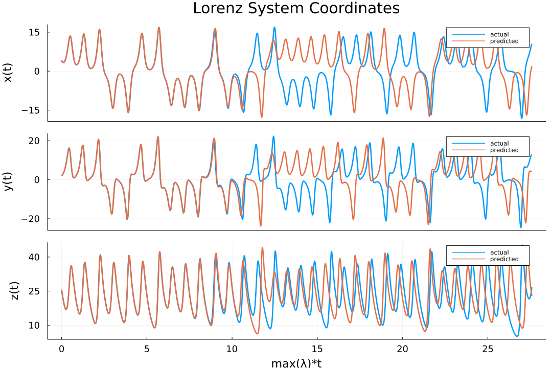

One can also visualize the phase space of the attractor and the comparison with the actual one:

plot(transpose(output)[:, 1],
    transpose(output)[:, 2],
    transpose(output)[:, 3],
    label = "predicted")
plot!(transpose(test)[:, 1], transpose(test)[:, 2], transpose(test)[:, 3], label = "actual")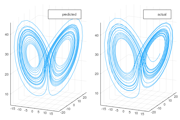

Citing

If you use this library in your work, please cite:

@article{JMLR:v23:22-0611,
  author  = {Francesco Martinuzzi and Chris Rackauckas and Anas Abdelrehim and Miguel D. Mahecha and Karin Mora},
  title   = {ReservoirComputing.jl: An Efficient and Modular Library for Reservoir Computing Models},
  journal = {Journal of Machine Learning Research},
  year    = {2022},
  volume  = {23},
  number  = {288},
  pages   = {1--8},
  url     = {http://jmlr.org/papers/v23/22-0611.html}
}

Acknowledgements

This project was possible thanks to initial funding through the Google summer of code 2020 program. Francesco M. further acknowledges ScaDS.AI and RSC4Earth for supporting the current progress on the library.