![]() (Testing is done with the latest stable release of Julia, on Linux, Windows, and MacOS)
(Testing is done with the latest stable release of Julia, on Linux, Windows, and MacOS)
Click on the following image to see an explanatory video:
A package for Bayesian Method of Simulated Moments estimation, following Kim, Jae-Young. "Limited information likelihood and Bayesian analysis." Journal of Econometrics 107.1-2 (2002): 175-193 and Chernozhukov, Victor, and Han Hong. "An MCMC approach to classical estimation." Journal of econometrics 115.2 (2003): 293-346. These methods are similar to some forms of Approximate Bayesian Computing.
The innovation is that the moment conditions are based on statistics that are filtered through a trained neural net, so that the filtered moments are exactly identifying. The methods lead to reliable inferences, in the sense that confidence intervals or credible intervals based on quantiles of MCMC chains contain true parameters at a proportion close to the nominal level, in addition to point estimators having low bias and RMSE. The evidence to support these claims is in the papers "Neural nets for indirect inference", Econometrics and Statistics, 2017, https://doi.org/10.1016/j.ecosta.2016.11.008 and "Inference Using Simulated Neural Moments" Econometrics, 2021, https://doi.org/10.3390/econometrics9040035.
The net is trained using many simulated draws from the prior, to get parameters, and the statistics resulting from a sample from the model at each parameter draw. With a large set of draws of parameter/statistics, the net is trained, using the statistics as the inputs, and the parameters as the outputs, using the Flux.jl machine learning package.
With a trained net, we can feed in statistics computed from real data, and obtain estimates of the parameters that generated the statistics. These estimated parameters then used as the statistics upon which ABC/MSM is based.
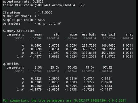
ABC/MSM draws from the posterior are done using MCMC with Metropolis-Hastings sampling. The proposal density is the same as the likelihood, but estimated at the point estimate from the net that corresponds to the real data. Because the proposal and the likelihood are of the same form, random walk MH sampling is effective for this application.
Please see the docs, in the link at the top, and the README for the two examples to see how this all works.